Main Goal:

• Learn the fundamental knownledge and mathmatical theory of Trajectory Generation in manipulator.
• Demo Python code of Trajectory Generation.

I. What is Trajectory Generation

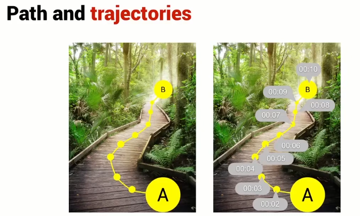
During robot motion, the robot controller receives a continuous stream of goal positions and velocities to track. This specification of the robot’s position as a function of time is called a trajectory. In some cases, the trajectory is completely determined by the task, such as when the end-effector needs to track a known moving object. In other cases, when the task is simply to move from one position to another in a given time, we have the freedom to design the trajectory to meet these constraints. This is the domain of trajectory planning. A trajectory should be a sufficiently smooth function of time and should respect any given limits on joint velocities, accelerations, or torques. We can consider a trajectory as the combination of a path, which is a purely geometric description of the sequence of configurations achieved by the robot, and a time scaling , which specifies the times when those configurations are reached. There are three cases to consider in trajectory planning:

1. Point-to-point straight-line trajectories in both joint space and task space.
2. Trajectories passing through a sequence of timed via points.
3. Minimum-time trajectories along specified paths, taking actuator limits into consideration

Definition

A path \(\theta(s)\) maps a scalar path parameter \(s\), assumed to be 0 at the start of the path and 1 at the end, to a point in the robot’s configuration space \(\Theta\),

As \(s\) increases from 0 to 1, the robot moves along the path. Sometimes \(s\) is taken to be time and is allowed to vary from time \(s = 0\) to the total motion time \(s = T\), but it is often useful to separate the role of the geometric path parameter \(s\) from the time parameter \(t\). A time scaling \(s(t)\) assigns a value \(s\) to each time \(t \in [0, T]\), \(s : [0, T] \rightarrow [0, 1]\).

Together, a path and a time scaling define a trajectory \(\theta(s(t))\), or \(\theta(t)\) for short. Using the chain rule, the velocity and acceleration along the trajectory can be written as

To ensure that the robot’s acceleration (and therefore dynamics) is well defined, each of \(\theta(s)\) and \(s(t)\) must be twice differentiable.

1. Point-to-Point Trajectories

The simplest type of motion is from rest at one configuration to rest at another, which is called point-to-point motion. For point-to-point motion, the simplest type of path is a straight line

1.1 Straight-Line Paths

Straight-line path in configuration space

A “straight line” from a start configuration \(\theta_{\text{start}}\) to an end configuration \(\theta_{\text{end}}\) could be defined in joint space or in task space. The advantage of a straight-line path from \(\theta_{\text{start}}\) to \(\theta_{\text{end}}\) in joint space is simplicity: since joint limits typically take the form \(\theta_{i,\text{min}} \leq \theta_i \leq \theta_{i,\text{max}}\) for each joint \(i\), the allowable joint configurations form a convex set \(\Theta_{\text{free}}\) in joint space, so the straight line between any two endpoints in \(\Theta_{\text{free}}\) also lies in \(\Theta_{\text{free}}\). The straight line can be written as:

\(\theta(s) = \theta_{\text{start}} + s(\theta_{\text{end}} - \theta_{\text{start}})\) ,

with derivatives:

Straight lines in joint space generally do not yield straight-line motion of the end-effector in task space.

Straight-line path in cartesian space

If task-space straight-line motions are desired, the start and end configurations can be specified by \(X_{\text{start}}\) and \(X_{\text{end}}\) in task space. If \(X_{\text{start}}\) and \(X_{\text{end}}\) are represented by a minimum set of coordinates, then a straight line is defined as:

Compared with the case when joint coordinates are used, the following issues must be addressed:

• If the path passes near a kinematic singularity, the joint velocities may become unreasonably large for almost all time scalings of the path.
• Since the robot’s reachable task space may not be convex in \(X\) coordinates, some points on a straight line between two reachable endpoints may not be reachable.

So a configuration of the form

does not generally lie in SE(3) -> Solution by using screw motion (simultaneous rotation about and translation along a fixed screw axis)

To derive this \(X(s)\), we can write the start and end configurations explicitly in the {s} frame as \(X_{s,\text{start}}\) and \(X_{s,\text{end}}\) and use our subscript cancellation rule to express the end configuration in the start frame: \(X_{\text{start},\text{end}} = X_{\text{start},s} X_{s,\text{end}} = X_{s,\text{start}}^{-1} X_{s,\text{end}}.\)

Then \(\log(X_{s,\text{start}}^{-1} X_{s,\text{end}})\) is the matrix representation of the twist, expressed in the {start} frame, that takes \(X_{\text{start}}\) to \(X_{\text{end}}\) in unit time. The path can therefore be written as \(X(s) = X_{\text{start}} \exp(\log(X_{\text{start}}^{-1} X_{\text{end}})s),\)

where \(X_{\text{start}}\) is post-multiplied by the matrix exponential since the twist is represented in the {start} frame, not the fixed world frame {s}.

This screw motion provides a “straight-line” motion in the sense that the screw axis is constant. The origin of the end-effector does not generally follow a straight line in Cartesian space, since it is following a screw motion. It may be preferable to decouple the rotational motion from the translational motion. Writing \(X = (R, p)\), we can define the path

where the frame origin follows a straight line while the axis of rotation is constant in the body frame. Figure bellow

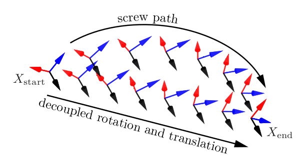
illustrates a screw path and a decoupled path for the same \(X_{\text{start}}\) and \(X_{\text{end}}\).

Example

(Left) A 2R robot with joint limits \(0^\circ \leq \theta_1 \leq 180^\circ\), \(0^\circ \leq \theta_2 \leq 150^\circ\). (Top center) A straight-line path in joint space and (top right) the corresponding motion of the end-effector in task space (dashed line). The reachable endpoint configurations, subject to joint limits, are indicated in gray. (Bottom center) This curved line in joint space and (bottom right) the corresponding straight-line path in task space (dashed line) would violate the joint limits.

• Cubic Path: A method of defining a geometric curve for the end-effector between two points using a cubic polynomial (3rd orders)

• Polynomial Path: A method of defining a geometric curve for the end-effector between two points using a polynomial, example Quintic path (5th orders). This method is also used to create smooth and continuous curves for robot motion.

• Non-polynomial Path Planning: A method of defining a geometric curve for the end-effector between two points using non-polynomial equations. This method is used to create smooth and continuous curves for robot motion.

• Forward Path Robot Motion: A method of controlling the motion of a robot by specifying the desired path of the end-effector. This method is used to move the robot from its current position to a desired position.

• Inverse Path Robot Motion: A method of controlling the motion of a robot by specifying the desired path of the end-effector and calculating the required joint angles to achieve that path. This method is used to move the robot from its current position to a desired position while avoiding obstacles.

• Rotational Path: A method of defining a path for a robot that involves rotation around a fixed point. This method is used to create circular or spiral paths for robot motion.

II. Mathematical form of each methods

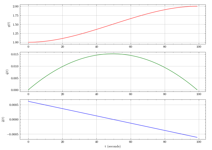
• Cubic Path: A method of defining a geometric curve for the end-effector between two points using a cubic polynomial. This method is used to create smooth and continuous curves for robot motion.

generates four equations for the coefficients of the path.

In case that \(t_0=0\), the coefficients simplify.

It is also possible to employ a time shift and search for a cubic polynomial of \(\left(t-t_0\right)\).

Now, the boundary conditions \(t_0 =0\) generate a set of equations

In this equation, \(p(t)\) represents the position of the end-effector at time \(t\), \(a_0\) represents the initial position of the end-effector, \(a_1\) represents the initial velocity of the end-effector, and \(a_2\) and \(a_3\) are the coefficients of the cubic polynomial. These coefficients are calculated using the initial and final conditions of the path, including the position, velocity, and acceleration.

Snippet code of Cubic_Path in Python:

Cubic_Path.py

import numpy as np
import matplotlib.pyplot as plt
import scienceplots


class Trajectory:
    """
    Trajectory class
    """
    def __init__(self, t,  q, qd, qdd):
        self.t = t
        self.q = q
        self.qd = qd
        self.qdd = qdd

    def plot(self):
        with plt.style.context(['science', 'no-latex', 'high-vis']):
            ax = plt.subplot(3, 1, 1)
            ax.grid(True)
            ax.plot(self.t, self.q, 'r')
            print("q: ", self.q)
            ax.set_ylabel("$(t)$")
            ax = plt.subplot(3, 1, 2)
            ax.grid(True)
            ax.plot(self.t, self.qd, 'g')
            ax.set_ylabel("$\dot(t)$")
            ax = plt.subplot(3, 1, 3)
            ax.grid(True)
            ax.plot(self.t, self.qdd, 'b')
            ax.set_ylabel(f"$\ddot(t)$")
            ax.set_xlabel("t (seconds)")
            plt.show()

def cubic(q0, qf, t, qd0=0, qdf=0):
    """
    cubic funtion 
    """
    if isinstance(t, int):
        t = np.arange(0, t)
        print("t: ", t)
    tf = max(t)
    polyfunc = cubic_func(q0, qf, tf, qd0, qdf)
    trajec = polyfunc(t)
    p   = trajec[0]
    pd  = trajec[1]
    pdd = trajec[2]
    return Trajectory(t, p , pd, pdd)

def cubic_func(q0, qf, T, qd0=0, qdf =0):
    """
    cubic function
    """
    A = [
        [ 0.0,      0.0,        0.0,      1.0],
        [ T**3,     T**2,       T,        1.0], 
        [ 0.0,      0.0,        1,        0.0],
        [3*T**2,    2*T,        1.0,      0.0],
    ]
    b = np.r_[q0, qf, qd0, qdf]
    # calculate coefficients by using  
    # least-squares solution to a linear matrix equation
    # A @ x = b -> find x 
    coeffs, resid, rank, s = np.linalg.lstsq(A, b , rcond=None)

    # coefficients of derivatives
    coeffs_d = coeffs[0:3] * np.arange(3, 0, -1)
    coeffs_dd = coeffs_d[0:2] * np.arange(2, 0, -1)

    return lambda t: (
        np.polyval(coeffs, t),
        np.polyval(coeffs_d, t),
        np.polyval(coeffs_dd, t),
    )

cubic_1 = cubic(1, 2, 100)
cubic_1.plot()

References

1. Reza N. Jazar. 2007. Theory of Applied Robotics: Kinematics, Dynamics, and Control. Springer Publishing Company, Incorporated.
2. Kevin M. Lynch and Frank C. Park. 2017. Modern Robotics: Mechanics, Planning, and Control (1st. ed.). Cambridge University Press, USA.
3. Professor Peter Corke, Robot Academy, https://robotacademy.net.au/lesson/summary-of-paths-and-trajectories/